EIDORS: Electrical Impedance Tomography and Diffuse Optical Tomography Reconstruction Software

Hosted by

2D Geophysical models with Distmesh

Create fine mesh

% Geophysics model $Id: dm_geophys01.m 1535 2008-07-26 15:36:27Z aadler $

n_nodes= 1000;
z_contact= 0.01;
n_elec= 9;
nodes_per_elec= 5;
elec_width= 0.2;
elec_spacing= 1.0;

xllim=-10; xrlim= 10; ydepth=-10;
xgrid=  linspace(-elec_width/2, +elec_width/2, nodes_per_elec)';
x2grid= elec_width* [-5,-4,-3,3,4,5]'/4;
refine_nodes= [xllim,0; xrlim,0; 0, ydepth];
for i=1:n_elec
% Electrode centre
  x0= (i-1-(n_elec-1)/2)*elec_spacing;
  y0=0;
  elec_nodes{i}= [x0+ xgrid, y0+0*xgrid];
  refine_nodes= [ refine_nodes; ...
                 [x0 + x2grid   ,  y0             + 0*x2grid];
                 [x0 + xgrid*1.5,  y0-elec_width/2+ 0*xgrid];
                 [x0 + x2grid*1.5, y0-elec_width/2+ 0*x2grid];
                 [x0 + xgrid*2   , y0-elec_width  + 0*xgrid];
                 [x0 + xgrid*2   , y0-elec_width*2+ 0*xgrid]];
end
  
% Distance to edge
%fd=inline('-min([10+p(:,1),10-p(:,1),-p(:,2),10+p(:,2)],[],2)','p');
fd=inline('-min(-p(:,2),10-sqrt(sum(p.^2,2)))','p');
bbox = [xllim,ydepth;xrlim,0];
gmdl= dm_mk_fwd_model( fd, [], n_nodes, bbox, ...
                          elec_nodes, refine_nodes, z_contact);


% Refine elements near upper boundary
n_nodes= 3000;
fh=inline('min(0.5-p(:,2)/4,2)','p');
fmdl= dm_mk_fwd_model( fd, fh, n_nodes, bbox, ...
                          elec_nodes, refine_nodes, z_contact);

% Show results - big
subplot(121)
show_fem(gmdl); axis on
subplot(122)
show_fem(fmdl); axis on

print -dpng -r150 dm_geophys01a.png

% Show results - small
subplot(121)
show_fem(gmdl); axis([-3,3,-3,0.3]);
subplot(122)
show_fem(fmdl); axis([-3,3,-3,0.3]);
print -dpng -r150 dm_geophys01b.png

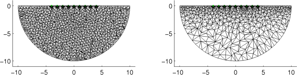
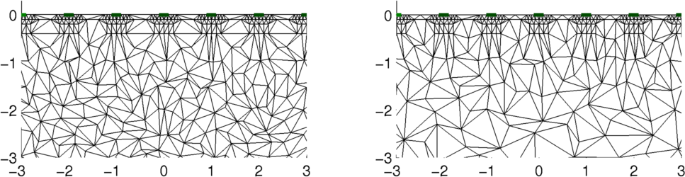
Figure: Geophysical model with electrodes on surface from distmesh Left: Uniform mesh density Right: Mesh density refined going from surface to bottom

Create rectangular coarse mesh

% Create and show square model $Id: dm_geophys02.m 1535 2008-07-26 15:36:27Z aadler $

% Create square mesh model
imdl= mk_common_model('c2s',16);
cmdl= rmfield(imdl.fwd_model,{'electrode','stimulation'});

% magnify and move down onto geophysics model
cmdl.nodes(:,2)= cmdl.nodes(:,2) - 1.05;
cmdl.nodes= cmdl.nodes*4;

% assign one parameter to each square
e= size(cmdl.elems,1);
params= ceil(( 1:e )/2);
cmdl.coarse2fine = sparse(1:e,params,1,e,max(params));

clf;
show_fem(fmdl);
hold on;
h= trimesh(cmdl.elems,cmdl.nodes(:,1),cmdl.nodes(:,2));
set(h,'Color',[0,0,1],'LineWidth',2);
hold off
axis image

print -dpng -r125 dm_geophys02a.png

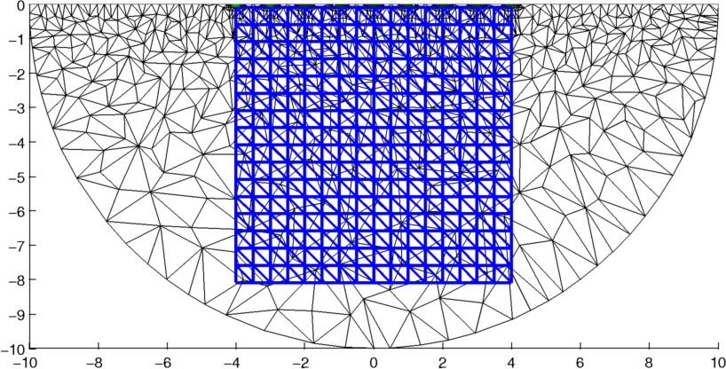
Figure: Coarse mesh (blue) superimposed onto the fine mesh (black). Electrode positions are shown in green.

Simulate Target

% simulate targets $Id: dm_geophys03.m 1535 2008-07-26 15:36:27Z aadler $

fmdl.stimulation= mk_stim_patterns(n_elec, 1, '{ad}','{ad}', {}, 1);

img= eidors_obj('image','fmdl','fwd_model',fmdl, ...
                'elem_data', ones(size(fmdl.elems,1),1) );
vh= fwd_solve(img);

% interpolate onto mesh
xym= interp_mesh( fmdl, 3);
x_xym= xym(:,1,:); y_xym= xym(:,2,:);
ff  = (x_xym>-2) & (x_xym<-1) & (y_xym<-2) & (y_xym>-3);
ff = mean(ff,3);
img.elem_data= img.elem_data + ff;

% inhomogeneous image
vi= fwd_solve(img);

show_fem(img); axis image;
print -dpng -r125 dm_geophys03a.png

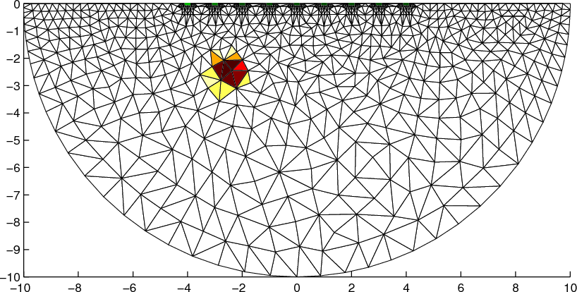
Figure: Simulated position of target in the fine mesh

Reconstruct image using dual model

% 2D solver $Id: dm_geophys04.m 1535 2008-07-26 15:36:27Z aadler $

% Create a new inverse model, and set
% reconstruction model and fwd_model
imdl= mk_common_model('c2c2',16);
imdl.rec_model= cmdl;
imdl.fwd_model= fmdl;

c2f= mk_coarse_fine_mapping( fmdl, cmdl);
imdl.fwd_model.coarse2fine = c2f;
imdl.RtR_prior = @gaussian_HPF_prior;
imdl.solve = @aa_inv_solve;
imdl.hyperparameter.value= 0.0001;

imgs= inv_solve(imdl, vh, vi);

show_fem(fmdl); ax= axis;
hold on
show_fem(imgs);
hold off
axis(ax); axis image
print -dpng -r125 dm_geophys04a.png

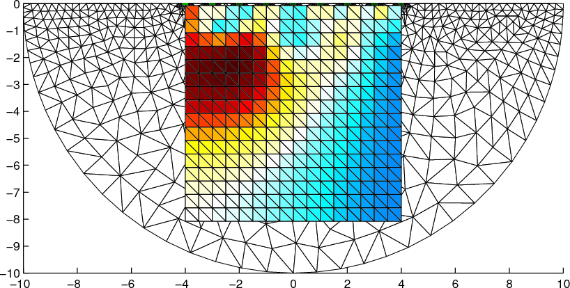
Figure: Reconstructed target showing coarse and fine mesh in background.