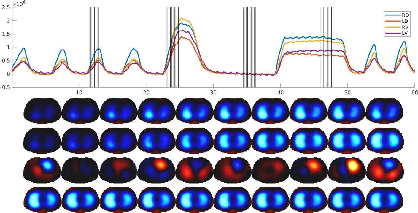
Top: Waveforms in regions of interest vs time (s). Bottom: Image sequences corresponding to vertical line segments in the data.
| Authors: | Eckhard Teschner
|
|---|---|
| Date: | 2024-02-27
|
| Brief Description: |
Recordings in a healthy subject with the Draeger PulmoVista 500, SW1.30: regular breathing followed by +expiratory and inspiratory breath holds.
|
| License: | Creative Commons License: CC-ND
|
| Attribution Requirement: | Attribution is not required. |
| Format: | Data files are stored in the PulmoVista 500 *.eit format and the MCEIT *.get format. Fraame rate is 20 frames/sec.
|
| Methods: |
The subject (healthy adult male) was seated with the Draeger PulmoVista 500
belt in the recommended position (4th to 5th intercostal space at the
midclavicular line). EIT measurements were performed while the subject
performed tidal breathing, followed by a deeper breath, as well as a short
expiratory and inspiratory breath hold.
|
| Data: | Data (Draeger EIT format)
Data (MCEIT GET format) |
file = 'ET_Test_File_Healthy_Lung_01';
% Load data in Draeger format
 [dd,aux]= eidors_readdata([file,'.eit']);     opt = 'rotate_meas';
% Load data in MCEIT get format
%[dd,aux]= eidors_readdata([pth,'_01.get']); opt = 'no_rotate_meas';

% Set fwd model parameters
fmdl = mk_library_model('adult_male_32el'); fmdl.electrode(1:2:end)=[];
fmdl.frame_rate = aux.frame_rate;
[fmdl.stimulation,fmdl.meas_select]= mk_stim_patterns(16,1,[0,1],[0,1],{opt});

% Normalized and non-normalized reconstruction with Draeger data are both possible.
%fmdl.normalize_measurements= true;
imdl = select_imdl(fmdl,{'GREIT:NF=0.3 64x64 rad=0.25'});

[ROIs,imgR] = define_ROIs(imdl,[-2,0,2],[-2,0,2]);
imgr = inv_solve(imdl, mean(dd,2), dd);
% choose reference between t=33 and t=37
dh = mean(dd(:,abs(imgr.time-35)<2),2);
imgr = inv_solve(imdl, dh, dd);

subplot(311);
plot(imgr.time,-(ROIs*imgr.elem_data)','LineWidth',2);
box off; yl=ylim;
legend('RD','LD','RV','LV','AutoUpdate','off');

imgr.show_slices.img_cols = 10;
imgr.calc_colours = struct('backgnd',[1,1,1],'greylev',0.1);
imgr.calc_colours.ref_level = 0;

% Show image sequences
for sp=3:6; subplot(6,1,sp);
  idx = (sp-2)*230 + (0:9) * 4;
  imgr.get_img_data.frame_select = idx;
  show_slices(imgr);
  subplot(311);
  line([1;1]*imgr.time(idx),yl'*ones(1,10),'Color',[0,0,0]);
end
ylim(yl); axis tight
print_convert 'analyze01a.jpg' -p14x10