
|
|
EIDORS: Electrical Impedance Tomography and Diffuse Optical Tomography Reconstruction Software |
|
EIDORS
(mirror) Main Documentation Tutorials − Image Reconst − Data Structures − Applications − FEM Modelling − GREIT − Old tutorials − Workshop Download Contrib Data GREIT Browse Docs Browse SVN News Mailing list (archive) FAQ Developer
Hosted by |
Contrasts in EITIn EIT the contrast (signal change for a target) is not a uniform function of the conductivity. The effect is subtle and it is explored in this tutorial.Overview of EIT contrast signalHere we introduce a cylindrical contrast of various height/diameter axis ratios
% $Id: contrasts_06.m 5755 2018-05-19 11:03:13Z aadler $
[stim,msel] = mk_stim_patterns(16,1,[0,1],[0,1],{},1);
space= logspace(-3,3,37);
diam = 0.10;
i=1; vv=[]; for rat = [.3,1,2,5];
   extra={'targ',sprintf(['solid targ = ', ...
          'cylinder(0,0,0;0,0,1;%f) and ', ...
          'plane(0,0,%f;0,0,-1) and plane(0,0,%f;0,0,1);'], ...
           diam,diam*[-1,+1]*rat+1)};
   fmdl= ng_mk_cyl_models([2,1,.1],[16,1.0],[0.05],extra);
   fmdl.stimulation = stim; fmdl.meas_select = msel;
   img= mk_image(fmdl,1);
   vh = fwd_solve(img); vh = vh.meas;
   img.elem_data(fmdl.mat_idx{2}) = 2; show_fem(img);

   j=1;for k=space;
      img.elem_data(fmdl.mat_idx{2}) = k;
      vi = fwd_solve(img); vi = vi.meas;
      vv(j,i)= norm(vi-vh);
   j=j+1;end
i=i+1;end
vv = vv ./ (ones(size(vv,1),1)*max(vv,[],1));
clf; subplot(211);

opt.viewpoint = struct('az',-6,'el',13); show_fem_enhanced(img,opt);
print_convert contrasts_06a.jpg

%subplot(212);
semilogx(space,vv,'LineWidth',2);
legend('0.3','1.0','2.0','5.0','Location','SouthEast')
xlim([min(space), max(space)])
set(gca,'xtick',[1e-3,1e-2,1e-1,1,1e1,1e2,1e3]);
print_convert contrasts_06b.png
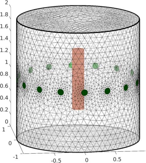

Figure: Left: 3D FEM with an ellipsoidal target region: Right: 3D FEM with an ellipsoidal target region: Creating an FEM and solving the forward problem
sz = 5;
ellipse_x = 2;

shape_str = [ ...
 sprintf('solid ec = ellipticcylinder(0,0,0;%f,0,0;0,%f,0);\n', ...
     0.5*ellipse_x, 0.5/ellipse_x ) ...
 sprintf('solid left  = plane(-%f,0,0;-1,0,0);\n',sz) ...
 sprintf('solid right = plane( %f,0,0; 1,0,0);\n',sz) ...
 sprintf('solid brick = orthobrick(-%f,-2,-0.2;%f,2,0);\n',sz+1,sz+1) ...
 'solid cyl = ec and brick; tlo cyl;\n' ...
 'solid mainobj= left and right and (not cyl) and brick;\n'];
elec_pos = [ sz,  0,  0,   0,  0,  1;
            -sz,  0,  0,   0,  0, -1];
elec_shape=[2.0];
elec_obj = {'left','right'};
fmdl = ng_mk_gen_models(shape_str, elec_pos, elec_shape, elec_obj);
fmdl = mdl2d_from3d(fmdl);

fmdl.stimulation = stim_meas_list([1,2,1,2]);
img = mk_image(fmdl,1);
img.elem_data( fmdl.mat_idx{1} ) = 2;

img.calc_colours.ref_level = 1;

show_fem( img );
print_convert contrasts_01a.png
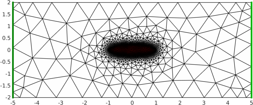
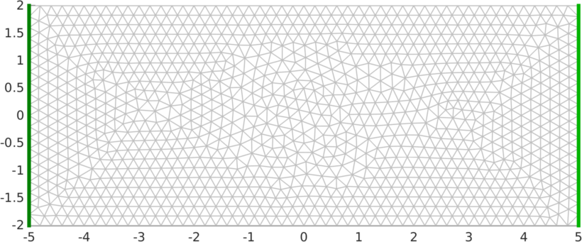
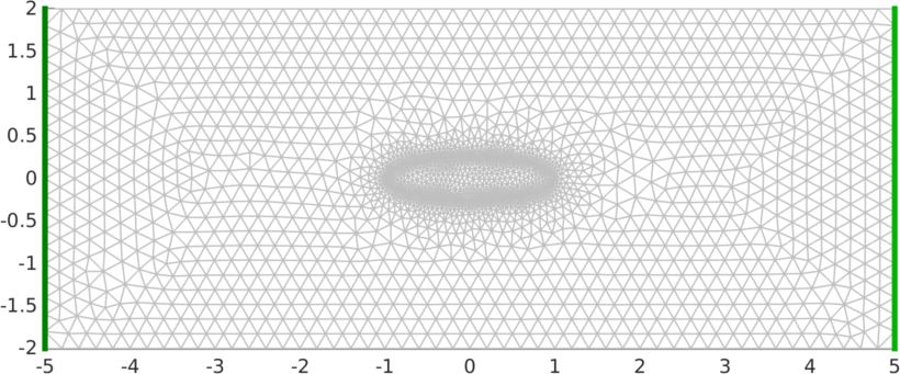
Figure: A 2D finite element model with an elliptical conductivity contrasting inclusion img.fwd_model.solve = @fwd_solve_1st_order; img.fwd_model.system_mat = @system_mat_1st_order; [img.fwd_model.electrode(:).z_contact] = deal(1000); % Large img.fwd_solve.get_all_meas = 1; vv = fwd_solve(img); imgv= rmfield(img,'elem_data'); imgv.node_data = vv.volt; imgv.calc_colours.ref_level = mean(vv.volt); show_fem(imgv); print_convert contrasts_02a.png 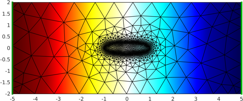
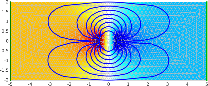
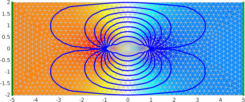
Figure: Voltage distribution around an elliptical conductivity with a conductive contrast
   imgc = img;
   imgc.fwd_model.mdl_slice_mapper.npx = 128;
   imgc.fwd_model.mdl_slice_mapper.npy = 200;
   imgc.fwd_model.mdl_slice_mapper.level = [inf,inf,0];
   imgc.calc_colours.ref_level = 1;
   q = show_current(imgc,vv.volt);

   fm1 = img.fwd_model;
   fm1.elems = fm1.elems(fm1.mat_idx{1},:);
   bdy= find_boundary(fm1);

   hh=show_fem(img.fwd_model);
   set(hh,'EdgeColor',[1,1,1]*.75);
   hold on;
   plot( reshape(fm1.nodes(bdy,1),size(bdy))', ...
         reshape(fm1.nodes(bdy,2),size(bdy))','k','LineWidth',2);

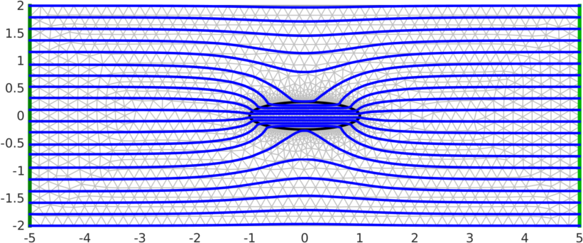
   sy = linspace(-2,2,20); sx= 0*sy - sz;
   hh=streamline(q.xp,q.yp, q.xc, q.yc,-sx,sy); set(hh,'Linewidth',2);

   hold off;

if ~exist('img_name'); img_name = '03a'; end
print_convert(sprintf('contrasts_%s.png',img_name));
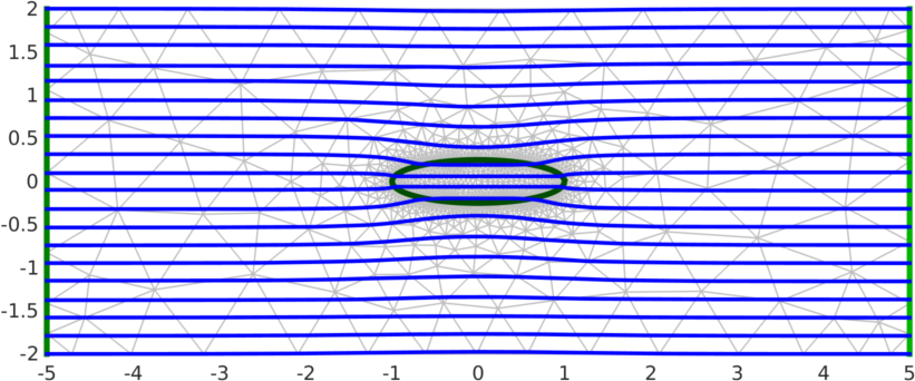
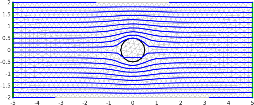
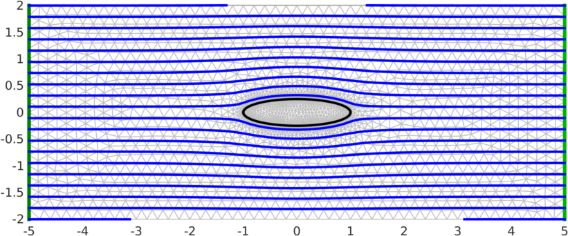
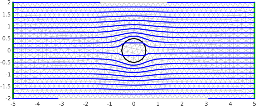
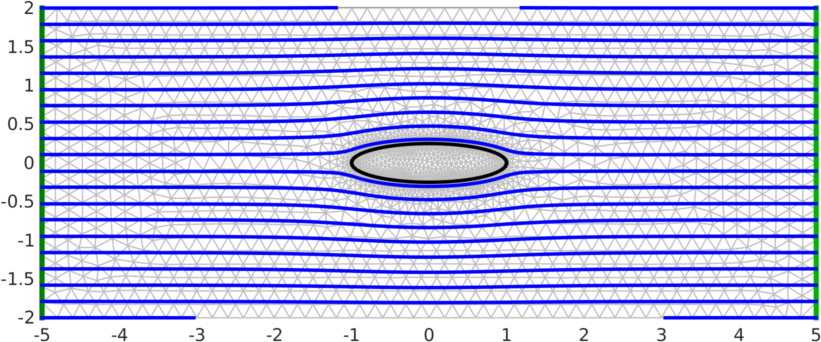
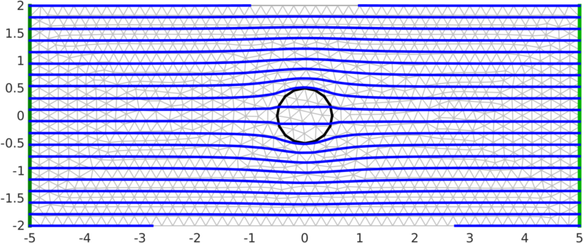
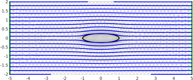
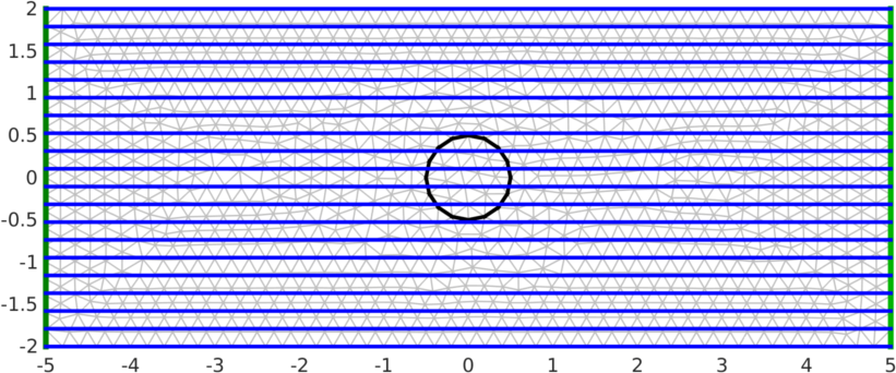
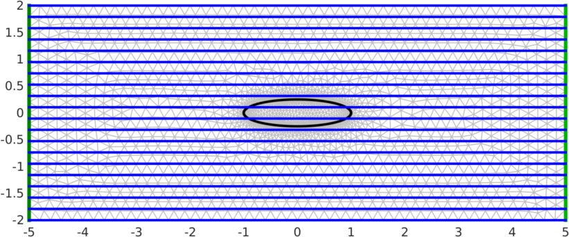
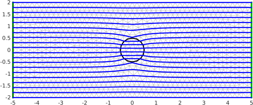
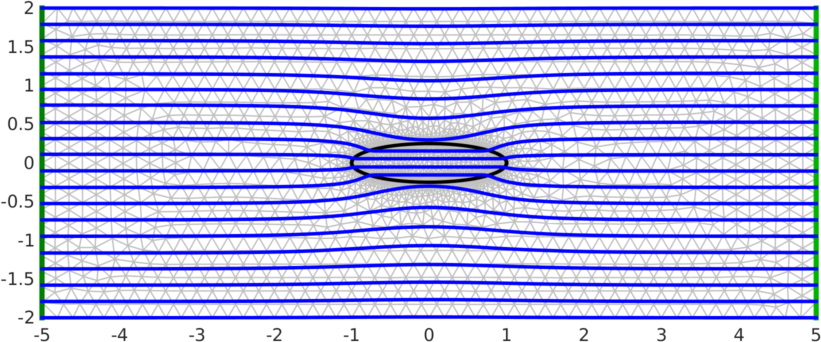
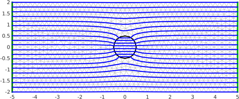
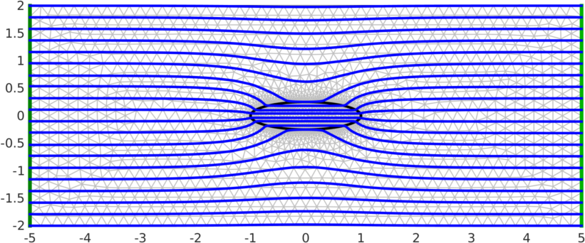
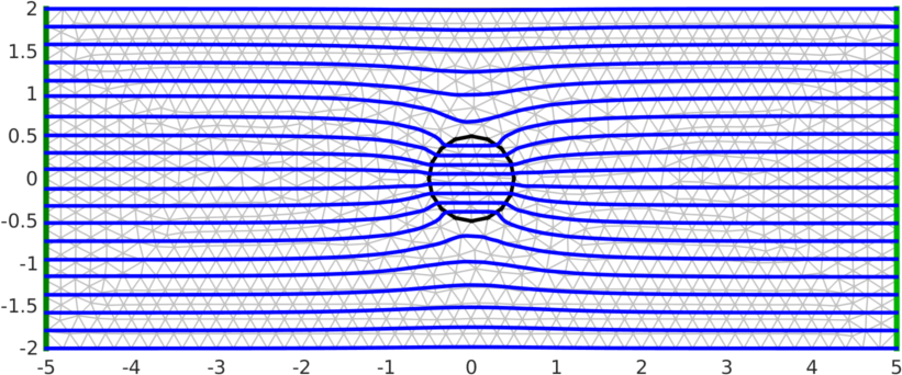
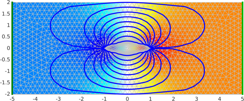
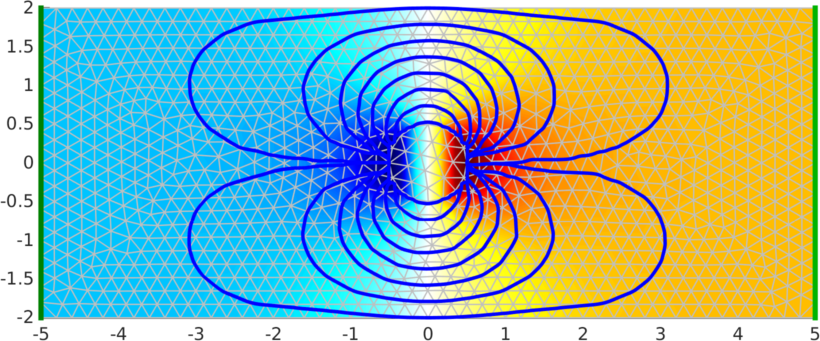
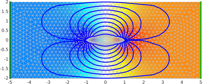
Figure: Streamlines around a conductive contrasting target |
function img = ellipse_in_plane( sz, ellipse_x);
   shape_str = [ ...
    sprintf('solid ec = ellipticcylinder(0,0,0;%f,0,0;0,%f,0);\n', ...
        0.5*ellipse_x, 0.5/ellipse_x ) ...
    sprintf('solid left  = plane(-%f,0,0;-1,0,0);\n',sz) ...
    sprintf('solid right = plane( %f,0,0; 1,0,0);\n',sz) ...
    sprintf('solid brick = orthobrick(-%f,-2,-0.2;%f,2,0) -maxh=0.2;\n',sz+1,sz+1) ...
    'solid cyl = ec and brick; tlo cyl;\n' ...
    'solid mainobj= left and right and (not cyl) and brick;\n'];
   elec_pos = [ sz,  0,  0,   0,  0,  1;
               -sz,  0,  0,   0,  0, -1];
   elec_shape=[2.0];
   elec_obj = {'left','right'};
   fmdl = ng_mk_gen_models(shape_str, elec_pos, elec_shape, elec_obj);
   fmdl = mdl2d_from3d(fmdl);

   fmdl.stimulation = stim_meas_list([1,2,1,2]);
   img = mk_image(fmdl,1);
   img.fwd_model.solve =      @fwd_solve_1st_order;
   img.fwd_model.system_mat = @system_mat_1st_order;
   [img.fwd_model.electrode(:).z_contact] = deal(1000); % Large
   img.fwd_solve.get_all_meas = 1;
Iterate over model shapes
sz = 5; img_idx = 'b';
for ellipse_x = [0.5,1,2];
   img = contrasts_04_modeller( sz, ellipse_x);
   targ = img.fwd_model.mat_idx{1};
   for contrast = linspace( -3,3,7);
      img.elem_data( targ ) = exp(contrast);
      vv = fwd_solve(img);
      img_name = sprintf('04%c',img_idx); img_idx= img_idx+1;
      contrasts_03;
   end
end
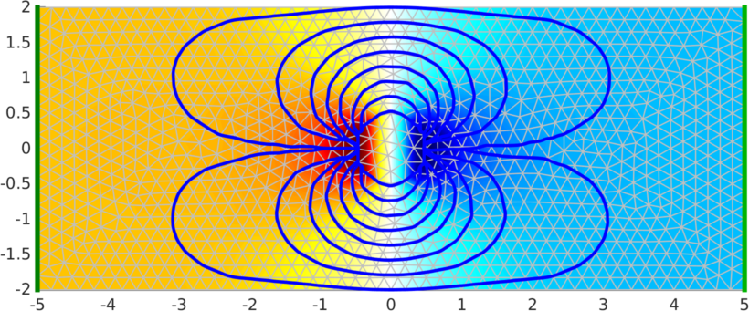
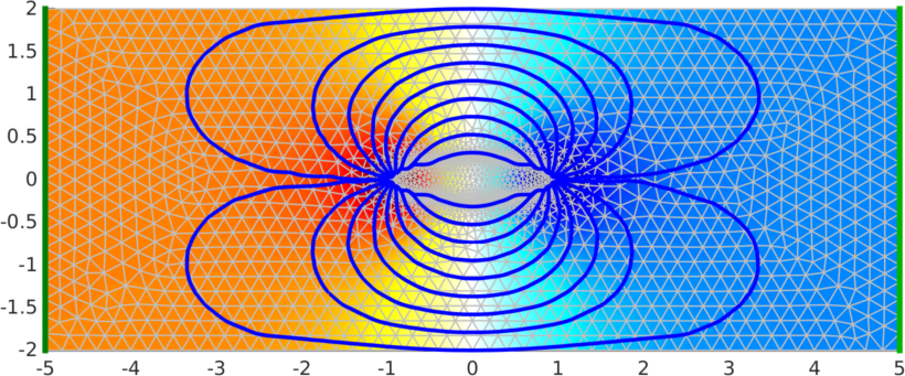
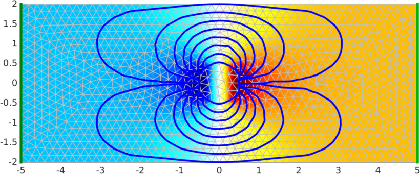
| σ = | x/y = 2 | x/y = 1 | x/y = ½ |
|---|---|---|---|
| e−3 | 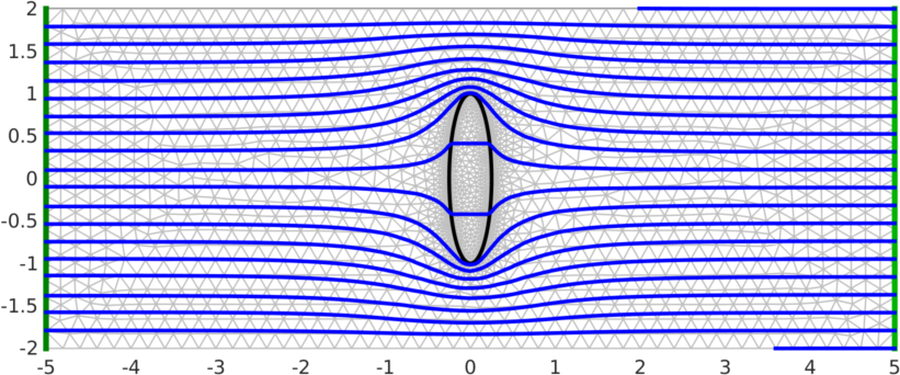
| 
| 
|
| e−2 | 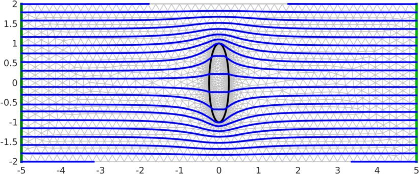
| 
| 
|
| e−1 | 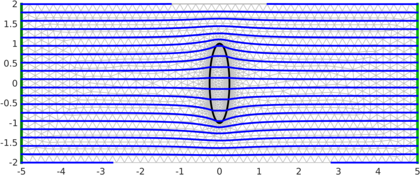
| 
| 
|
| e0 | 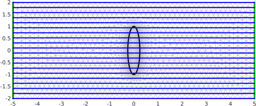
| 
| 
|
| e+1 | 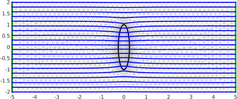
| 
| 
|
| e+2 | 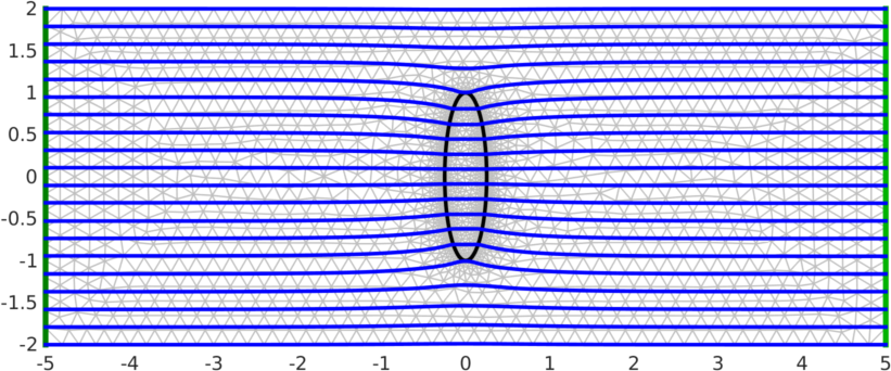
| 
| 
|
| e+3 | 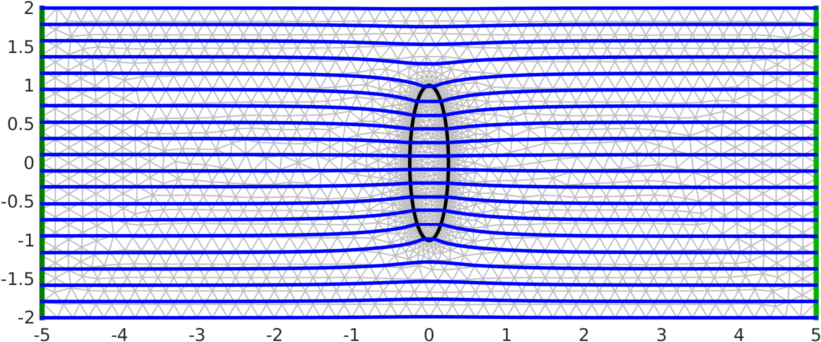
| 
| 
|
| σ = | x/y = 2 | x/y = 1 | x/y = ½ |
|---|---|---|---|
| e−2 | 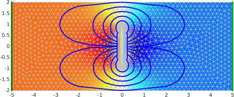
| 
| 
|
| e−1 | 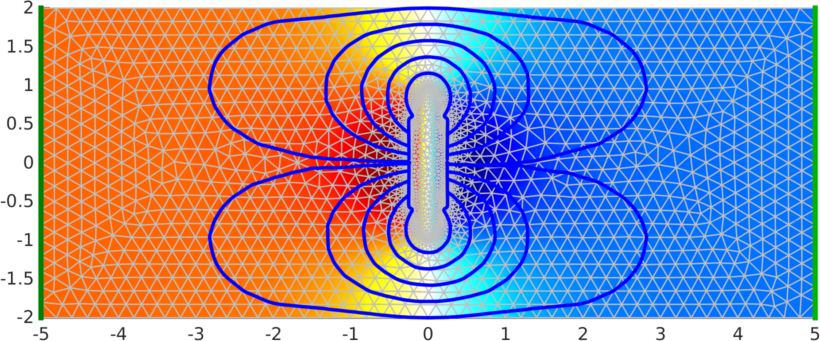
| 
| 
|
| e0 | 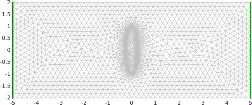
| 
| 
|
| e+1 | 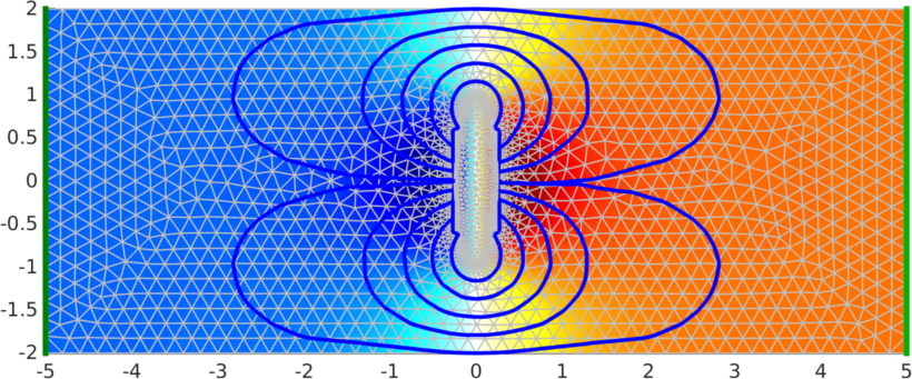
| 
| 
|
| e+2 | 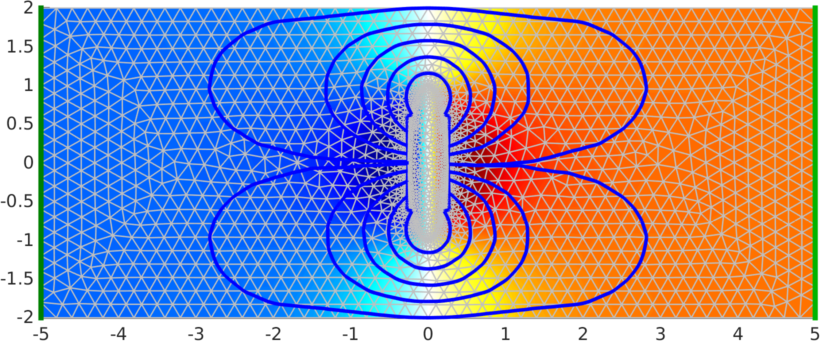
| 
| 
|
Last Modified: $Date: 2018-03-19 18:54:58 -0400 (Mon, 19 Mar 2018) $ by $Author: aadler $