EIDORS: Electrical Impedance Tomography and Diffuse Optical Tomography Reconstruction Software

Hosted by

Algorithm Performance

% Test algorithm performance $Id: algorithm_performance01.m 2240 2010-07-04 14:41:32Z aadler $

% Reconstruct GREIT Images
imdl_gr = mk_common_gridmdl('GREITc1');

% Reconstruct backprojection Images
imdl_bp = mk_common_gridmdl('backproj');

% Reconstruct GN Images
imdl_gn = select_imdl( mk_common_model('d2c2', 16), {'Basic GN dif','Choose NF=0.5'});

test_performance( { imdl_gr, imdl_bp, imdl_gn } );

print_convert 'algorithm_performance01a.png' '-density 100'

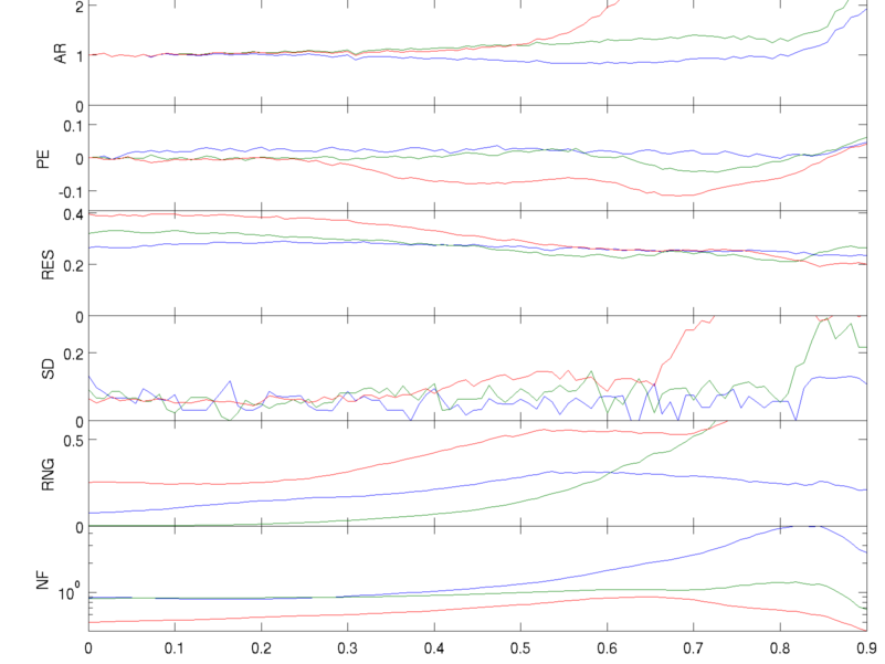
Figure: Performance of algorithms: blue: GREIT (v1) green: Sheffield backprojection red: One step Gauss Newton

GREIT Test Parameters for different algorithms

Simulate 3D object

% create 3D forward model
fmdl = ng_mk_cyl_models([2,1,0.08],[8,0.8,1.2],[0.05]); 
fmdl.stimulation = mk_stim_patterns(16,1,[0,1],[0,1],{},1);
imgs= mk_image( fmdl, 1);

show_fem(imgs);
print_convert test_params01a.png '-density 50'

Figure: Simulation mesh

Simulate target positions

r = 0.05; % target radius
Npos = 20; % number of positions
Xpos =  linspace(0,0.9,Npos); % positions to simulated along x-axis
Ypos = zeros(1,Npos); 
Zpos = ones(1,Npos);  %% for off-plane, adjust the level (*1.5)
xyzr = [Xpos; Ypos; Zpos; r*ones(1,Npos)];

[vh,vi] = simulate_movement(imgs, xyzr);

Gauss-Newton Reconstruction Matrix

% 3D inverse model
imdl= mk_common_model('n3r2',[16,2]);
mdl= ng_mk_cyl_models([2,1,0.1],[8,0.8,1.2],[0.05]); 
mdl.stimulation = mk_stim_patterns(16,1,[0,1],[0,1],{},1);
imdl.fwd_model = mdl; 

img= mk_image( mdl, 1); J = calc_jacobian(img);

%% inverse solution (faster solution)
hp  = 0.015;
RtR = prior_noser( imdl ); P= inv(RtR);
Rn = speye( size(J,1) );
imdl.solve = @solve_use_matrix;
imdl.solve_use_matrix.RM = P*J'/(J*P*J' + hp^2*Rn);
imgr= inv_solve(imdl,vh,vi);

Calculate and show GREIT parameters

%% calculate the GREIT parameters
levels =[inf,inf,Zpos(1)];
show_slices(imgr, levels);
imgr.calc_colours.npoints = 128;
imgr.calc_slices.levels=levels;
params = eval_GREIT_fig_merit(imgr, xyzr);

p_names = {'AR','PE','RES','SD','RNG'};
for i=1:5; subplot(5,1,i);
    plot(params(i,:)); ylabel(p_names{i});
end
print_convert test_params04a.png '-density 100'

Figure: GREIT figure of merit parameters for GN algorithm