EIDORS: Electrical Impedance Tomography and Diffuse Optical Tomography Reconstruction Software

Hosted by

Image reconstruction of moving objects

Andy Adler, Tao Dai, William R.B. Lionheart Temporal Image Reconstruction in Electrical Impedance Tomography Physiol. Meas., 2007.

Sample Data

Since the temporal solver works best for noisy data, we simulate a fairly low SNR (high NSR). To understand why the temporal solver works best at for noisy data, consider that if data are clean, then there is no reason to look at data from the past/future, since the current measurement tells us everything we need to know.

% Sample Data $Id: temporal_solver01.m 1535 2008-07-26 15:36:27Z aadler $

if ~exist('simulate_2d_movement_data.mat')
    [vh,vi,xyr_pt]=simulate_2d_movement;
    save simulate_2d_movement_data vi vh xyr_pt
else
    load simulate_2d_movement_data
end

% Temporal solver works best at large Noise
nsr= 4.0; %Noise to Signal Ratio

signal = mean( abs(mean(vi,2) - vh) ); % remember to define signal
% Only add noise to vi. This is reasonable, since we have
% lots of data of vh to average to reduce noise
vi_n= vi + nsr*signal*randn( size(vi) );

Reconstruction Algorithms

Over time steps, k, a sequence of difference vectors, y_k = Jx_k, are measured (assuming the body and electrode geometry, and thus J, stay fixed). If the conductivity of the body under investigation doesn’t change too rapidly, then it is reasonable to expect that a certain number of measurements, d, into the past and future provide useful information about the current image. Labelling the current instant as t, we therefore seek to estimate x_t from data [y_t-d; ... ; y_t-1; y_t; y_t+1; ... ; y_t+d].

In the subsequent sections we consider three traditional approaches and the proposed temporal inverse; each estimates x_t at frame t from a sequence of data starting at frame 0, using the indicated data:

1. Gauss-Newton (GN) inverse, using y_t only;
2. GN with weighted data, using a weighted average of y_t-d ... y_t+d;
3. Kalman filter inverse, using all previous and current data, y₀ ... y_t;
4. Temporal inverse, using y_t-d ... y_t+d based on a temporal prior model.

% Image reconstruction of moving objects $Id: temporal_solver02.m 1535 2008-07-26 15:36:27Z aadler $

time_steps=  3;
time_weight= .8;

base_model = mk_common_model( 'c2c2', 16 ); % 576 element
base_model.fwd_model.normalize_measurements= 0;
% HP value gives good solutions (calculated via Noise Figure)
hp= 0.101046;
base_model.hyperparameter.value= hp;

% GN Solver
imdl_GN = base_model;
imdl_GN.RtR_prior= @noser_image_prior;
imdl_GN.noser_image_prior.exponent= .5;
imdl_GN.solve= @np_inv_solve;
imdl_GN.hyperparameter.value= hp;
imdl_GN.fwd_model.normalize_measurements= 0;

% Temporal Solver
imdl_TS = base_model;
imdl_TS.RtR_prior= @time_smooth_prior;
imdl_TS.time_smooth_prior.space_prior= @noser_image_prior;
imdl_TS.noser_image_prior.exponent= .5;
imdl_TS.time_smooth_prior.time_weight= time_weight;
imdl_TS.time_smooth_prior.time_steps=  time_steps;
imdl_TS.solve= @time_prior_solve;
imdl_TS.time_prior_solve.time_steps=   time_steps;

% Kalman Solver
imdl_KS = base_model;
imdl_KS.RtR_prior= @noser_image_prior;
imdl_KS.noser_image_prior.exponent= .5;
imdl_KS.solve= @inv_kalman_diff;

Image Reconstruction

% Image reconstruction of moving objects $Id: temporal_solver02.m 1535 2008-07-26 15:36:27Z aadler $

time_steps=  3;
time_weight= .8;

base_model = mk_common_model( 'c2c2', 16 ); % 576 element
base_model.fwd_model.normalize_measurements= 0;
% HP value gives good solutions (calculated via Noise Figure)
hp= 0.101046;
base_model.hyperparameter.value= hp;

% GN Solver
imdl_GN = base_model;
imdl_GN.RtR_prior= @noser_image_prior;
imdl_GN.noser_image_prior.exponent= .5;
imdl_GN.solve= @np_inv_solve;
imdl_GN.hyperparameter.value= hp;
imdl_GN.fwd_model.normalize_measurements= 0;

% Temporal Solver
imdl_TS = base_model;
imdl_TS.RtR_prior= @time_smooth_prior;
imdl_TS.time_smooth_prior.space_prior= @noser_image_prior;
imdl_TS.noser_image_prior.exponent= .5;
imdl_TS.time_smooth_prior.time_weight= time_weight;
imdl_TS.time_smooth_prior.time_steps=  time_steps;
imdl_TS.solve= @time_prior_solve;
imdl_TS.time_prior_solve.time_steps=   time_steps;

% Kalman Solver
imdl_KS = base_model;
imdl_KS.RtR_prior= @noser_image_prior;
imdl_KS.noser_image_prior.exponent= .5;
imdl_KS.solve= @inv_kalman_diff;

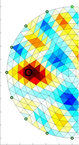
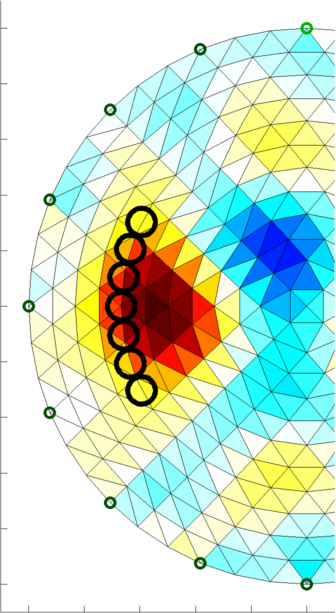
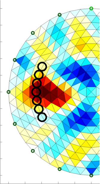
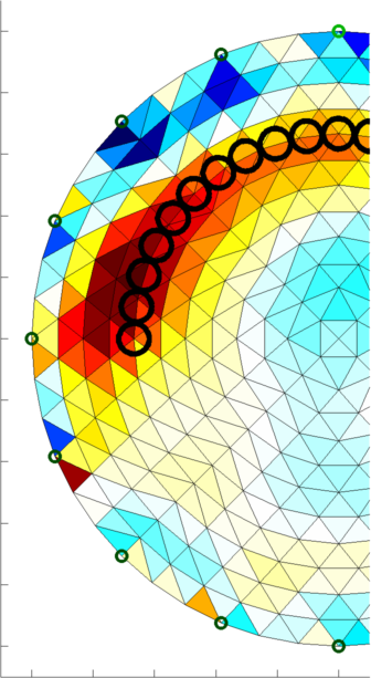
Figure: Image reconstructions of a moving ball in a medium. Top: using a classic one-stop solver, Bottom: using a Kalman solver. Note the warm up period of the Kalman images when the time correlations are being trained.

Image Reconstruction Movies

% Image reconstruction of moving objects $Id: temporal_solver04.m 1535 2008-07-26 15:36:27Z aadler $

time_steps=  3; ts_expand= 5;
time_weight= .8;
ts_vec= -time_steps:time_steps;

image_select= .25*length(xyr_pt)+1:ts_expand:.75*length(xyr_pt)+1;

% GN Solver
 vi_sel = vi(:,image_select);
 img= inv_solve( imdl_GN, vh, vi_sel);
 animate_reconstructions('temporal_solver04a', img);

% Temporal Solver
 k=1;
 for i= image_select
   vi_sel= vi(:,i+ts_vec);
   imgs= inv_solve( imdl_TS, vh, vi_sel);
   img.elem_data(:,k)= imgs.elem_data(:,1+time_steps);
   k=k+1;
 end
 animate_reconstructions('temporal_solver04c', img);


% Kalman Solver
 vi_sel = vi(:,image_select);
 img= inv_solve( imdl_KS, vh, vi_sel);
 animate_reconstructions('temporal_solver04d', img);