EIDORS: Electrical Impedance Tomography and Diffuse Optical Tomography Reconstruction Software

Hosted by

EIDORS fwd_models

Solving the forward problem for EIT in 2D with higher order finite elements

• M G Crabb. EIT Reconstruction Algorithms for Respiratory Intensive Care. PhD Thesis, University of Manchester, 2014.
• M G Crabb. Convergence study of 2D forward problem of electrical impedance tomography with high-order finite elements. Inverse Problems in Science and Engineering, 2016.

%Make an inverse model and extract forward model
imdl = mk_common_model('c2C0',16);
fmdl = imdl.fwd_model;

%Default EIDORS solver
%Make image of unit conductivity
img0 = mk_image(fmdl,1);
img0.fwd_solve.get_all_meas = 1; %Internal voltage
v0=fwd_solve(img0);
v0e=v0.meas; v0all=v0.volt; 


%High-order EIDORS solver
%Change default eidors solvers
fmdl.solve = @fwd_solve_higher_order;
fmdl.system_mat = @system_mat_higher_order;
fmdl.jacobian = @jacobian_adjoint_higher_order;

%Add element type
fmdl.approx_type    = 'tri3'; % linear
%Make an image and get voltages using high order solver
img1 = mk_image(fmdl,1);
img1.fwd_solve.get_all_meas = 1; %Internal voltage
v1 = fwd_solve(img1); 
v1e=v1.meas; v1all=v1.volt;


%Plot electrode voltages and difference
clf;subplot(211); plot([v0e,v1e,[v0e-v1e]*100]);
legend('0','1','(1-0) x 100'); xlim([1,100]);

print_convert forward_solvers_2d_high_order01a.png

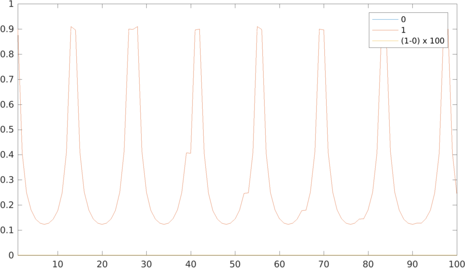
Figure: The plot reassuringly shows the two approximations (eidors default and the high order linear solver) both agree at machine precision on the electrodes.

%Get internal linear voltage distribution for first stimulation
v1all = v1.volt; 
img1n = rmfield(img1,'elem_data');
img1n.node_data = v1all(1:size(fmdl.nodes,1),1); %add first stim data

%Plot the distribution
img1n.calc_colours.cb_shrink_move = [0.5,0.5,0];
clf; subplot(221); show_fem(img1n,1);

%Get internal voltage distribution for difference eidors/high order
img11n=img1n; 
img11n.node_data=v1all(1:size(fmdl.nodes,1),1)-v0all(1:size(fmdl.nodes,1),1);

%Plot the difference of two linear approximations
img11n.calc_colours.cb_shrink_move = [0.5,0.5,0];
subplot(222); show_fem(img11n,1);

print_convert forward_solvers_2d_high_order02a.png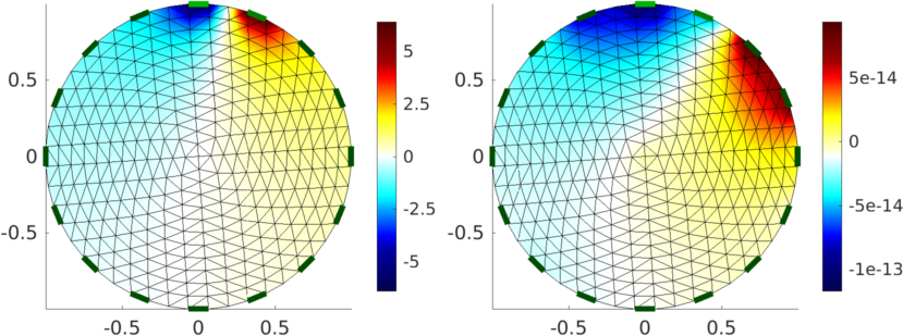

Figure: The left plot shows the voltage distribution for the first stimulation using the linear high order solver. The right plot shows the difference between the default eidors solver and the linear high order solver, which agree to machine precision.

%Repeat with quadratic and cubic finite elements
%Quadratic FEM
fmdl.approx_type    = 'tri6'; %Quadratic
img2 = mk_image(fmdl,1);
img2.fwd_solve.get_all_meas = 1; %Internal voltage
v2 = fwd_solve(img2); 
v2e=v2.meas; v2all=v2.volt;

%Cubic FEM
fmdl.approx_type    = 'tri10'; %Cubic
img3 = mk_image(fmdl,1);
img3.fwd_solve.get_all_meas = 1; %Internal voltage
v3 = fwd_solve(img3); 
v3e=v3.meas; v3all=v3.volt;

%Electrode voltages and difference for linear, quadratic and cubic
clf;subplot(211); plot([v1e,v2e,v3e,[v2e-v0e,v3e-v0e,v2e-v3e]*10]);
legend('1st order','2nd order','3rd order','(2-1) x 10','(3-1) x 10','(3-2) x 10')
xlim([1,100]);

print_convert forward_solvers_2d_high_order03a.png

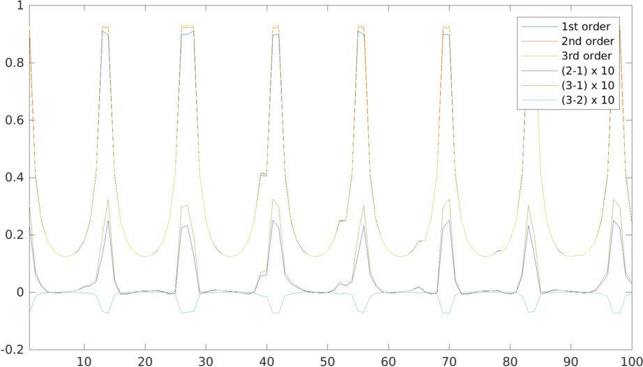
Figure: The electrode voltages for linear, quadratic and cubic approximation. The linear approximation agrees with the high order approximations away from the drive electrodes, but gets worse as we move toward the drive electrodes.

%Difference between quadratic and linear approximation internal voltage
img12n=img1n; 
img12n.node_data=v2all(1:size(fmdl.nodes,1),1)-v1all(1:size(fmdl.nodes,1),1);

%Plot the difference 
clf;
subplot(221); show_fem(img12n,1);
subplot(223); show_fem(img12n,1); axis([-0.2, 0.6, 0.3, 1.1]);

%Difference between quadratic and linear approximation internal voltage
img13n=img1n; 
img13n.node_data=v3all(1:size(fmdl.nodes,1),1)-v1all(1:size(fmdl.nodes,1),1);

%Plot the difference 
subplot(222); show_fem(img13n,1);
subplot(224); show_fem(img13n,1); axis([-0.2, 0.6, 0.3, 1.1]);

print_convert forward_solvers_2d_high_order04a.png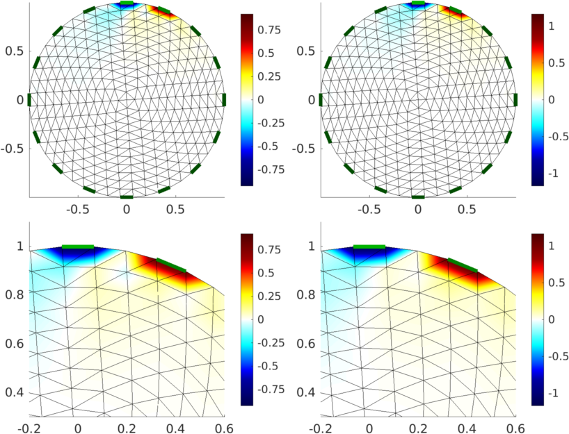

Figure: The left plot shows the difference between linear and quadratic approximation on the internal voltage distribution and the right plot shows the difference between linear and cubic approximation. The lower row shows a zoom into the upper plot

Iterate over model options (including solver and Jacobian)

imdl = mk_common_model('c2C',16); img = mk_image(imdl.fwd_model,1);
vv=fwd_solve(img);      v0e=vv.meas;
JJ=calc_jacobian(img);  J04=JJ(4,:)';

%High-order EIDORS solver %Change default eidors solvers
img.fwd_model.solve = @fwd_solve_higher_order;
img.fwd_model.system_mat = @system_mat_higher_order;
img.fwd_model.jacobian = @jacobian_adjoint_higher_order;

vve=[]; JJ4=[];
for i= 1:3; switch i;
   case 1; img.fwd_model.approx_type = 'tri3'; % linear
   case 2; img.fwd_model.approx_type = 'tri6'; % quadratic
   case 3; img.fwd_model.approx_type = 'tri10'; % cubic;
   end %switch
   vv=fwd_solve(img);      vve(:,i)=vv.meas;
   JJ=calc_jacobian(img);  JJ4(:,i)=JJ(4,:)';
end

subplot(311);
plot([v0e,vve,(v0e*[1,1,1]-vve)*10]);
legend('Default','linear','quadratic','cubic','(1-0)x10','(2-0)x10','(3-0)x10');
xlim([1,100]);

imgJJ=img; imgJJ.elem_data = JJ4;
imgJJ.show_slices.img_cols = 3;

subplot(312); show_slices(imgJJ); eidors_colourbar(imgJJ);

imgJJ.elem_data = JJ4 - J04*[1,1,1];
subplot(313); show_slices(imgJJ); eidors_colourbar(imgJJ);

print_convert forward_solvers_2d_high_order05a.png

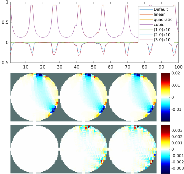
Figure: (top) plot of foward solutions and the differences between FEM orders (middle) a slice of the Jacobian for different FEM orders (bottom) difference between Jacobian values for different FEM orders