EIDORS: Electrical Impedance Tomography and Diffuse Optical Tomography Reconstruction Software

Hosted by

Using EIDORS to image gastric emptying

2D EIT for imaging of gastric emptying

Trudelle, Stéphane, Évaluation de la vidange gastrique par tomographie d'impédance électrique, Thesis (M.Sc.A.)--École polytechnique de Montréal

A. Adler, R. Guardo, Y. Berthiaume Imaging of Gastric Emptying with Electrical Impedance Tomography Canadian Medical and Biolological Eng. Soc., Vancouver, Canada, May 1994. 20:14-15.

Step 1: Create models

% Lung images
% $Id: tutorial410a.m 1535 2008-07-26 15:36:27Z aadler $

% 2D Model
imdl= mk_common_model('c2t3',16);


% most EIT systems image best with normalized difference
imdl.fwd_model.normalize_measurements= 1;
imdl.RtR_prior= @gaussian_HPF_prior;

% electrodes start on back (dorsal), then do this
imdl.fwd_model.electrode([9:16,1:8])=  ...
   imdl.fwd_model.electrode;


subplot(221);
show_fem(imdl.fwd_model);

axis equal
print -r100 -dpng tutorial410a.png;

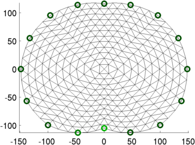
Figure: 2D FEM of thorax (units in mm). Electrode #1 (o) and electrode #2 (o) are shown in different colours than the others (o).

Image reconstruction

% Lung images
% $Id: tutorial410b.m 1535 2008-07-26 15:36:27Z aadler $

load montreal_data_1995
imdl.hyperparameter.value=5e-2;
vh= zc_h_stomach_pre; % abdomen before fluid
vi= zc_stomach_0_5_60min; % each 5 minutes after drink
img= inv_solve(imdl, vh, vi);

clf; show_slices(img)
axis equal

print -r100 -dpng tutorial410b.png;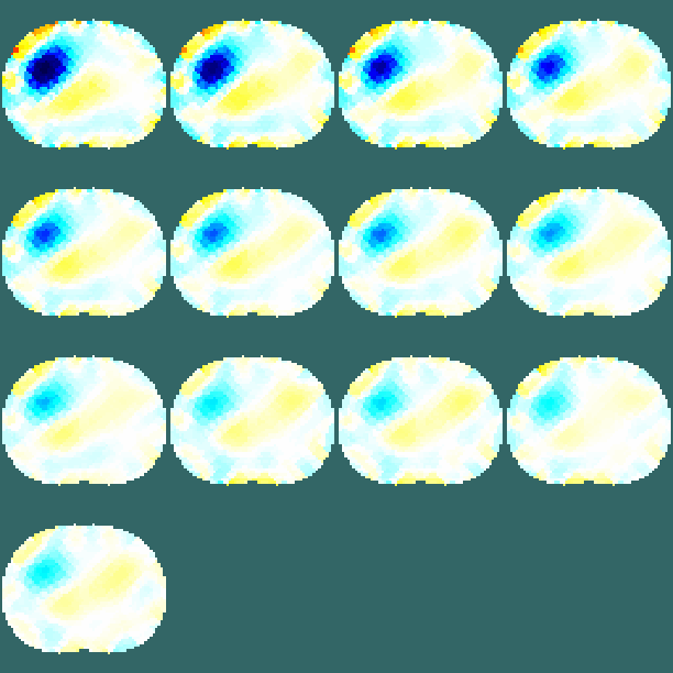

Figure: Image slices of the abdomen every five minutes after drink. Image progression is from left to right, top to bottom.

Calculate signal as a function of time

% Lung images
% $Id: tutorial410c.m 1535 2008-07-26 15:36:27Z aadler $

raster_img= calc_slices(img);
raster_img(isnan(raster_img))=0;
% define roi as whole image
s_ri = size(raster_img);
roi = ones(s_ri(1:2));

for i= 1:s_ri(3)
  sig(i)= sum(sum(raster_img(:,:,i) .* roi));
end

subplot(221)
plot( ((1:s_ri(3))-1)*5, sig/sig(1))
xlabel('minutes after drink')
ylabel('normalized conductivity');

print -r125 -dpng tutorial410c.png;

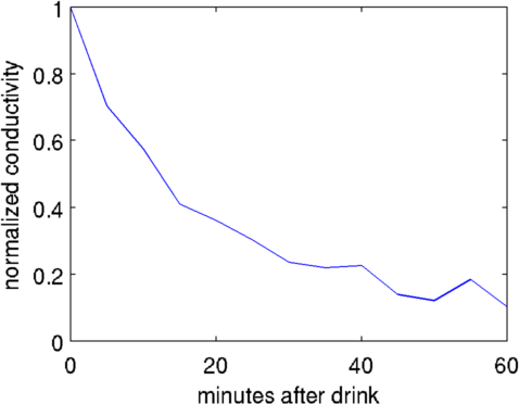
Figure: Normalized image in stomach as a function of time.

Different algorithms for stomach images

% Lung images
% $Id: tutorial410d.m 1535 2008-07-26 15:36:27Z aadler $

load montreal_data_1995
vh= zc_h_stomach_pre; % abdomen before fluid
vi= zc_stomach_0_5_60min(:,1); % right after drink

% GN solution - Gaussian prior
imdl.RtR_prior= @gaussian_HPF_prior;
imdl.solve=     @aa_inv_solve;
imdl.hyperparameter.value=1e-2;
img= inv_solve(imdl, vh, vi);

subplot(221); show_fem(img); axis equal; axis off

% GN solution - Noser prior
imdl.RtR_prior= @noser_image_prior;
imdl.solve=     @aa_inv_solve;
imdl.hyperparameter.value=8e-2;
img= inv_solve(imdl, vh, vi);

subplot(222); show_fem(img); axis equal; axis off

% GN solution - Noser prior
imdl= rmfield(imdl,'RtR_prior');
imdl.R_prior=   @ab_calc_tv_prior;
imdl.solve=     @ab_tv_diff_solve;
imdl.hyperparameter.value=1e-2;
img= inv_solve(imdl, vh, vi);

subplot(223); show_fem(img); axis equal; axis off

% GN solution - Noser prior
imdl.R_prior=   @ab_calc_tv_prior;
imdl.solve=     @ab_tv_diff_solve;
imdl.hyperparameter.value=1e-1;
img= inv_solve(imdl, vh, vi);

subplot(224); show_fem(img); axis equal; axis off


print -r100 -dpng tutorial410d.png;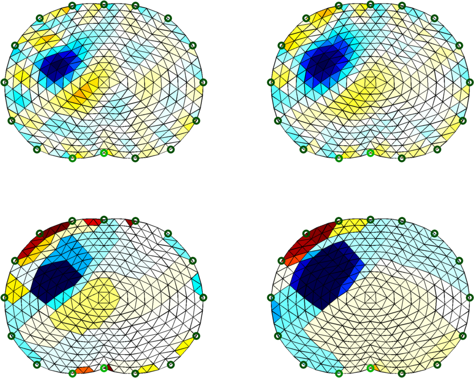

Figure: Top Left: Gauss-Newton Reconstruction with Gaussian HPF prior Top Right: Gauss-Newton Reconstruction with Laplacian filter Bottom Left: Total Variation Reconstruction (hp=1e-3) Bottom Right: Total Variation Reconstruction (hp=1e-4)